

Authors:
(1) Andrew Draganov, Aarhus University and All authors contributed equally to this research;
(2) David Saulpic, Université Paris Cité & CNRS;
(3) Chris Schwiegelshohn, Aarhus University.
Table of Links
2 Preliminaries and Related Work
2.3 Coresets for Database Applications
4 Reducing the Impact of the Spread
4.1 Computing a crude upper-bound
4.2 From Approximate Solution to Reduced Spread
5 Fast Compression in Practice
5.1 Goal and Scope of the Empirical Analysis
5.3 Evaluating Sampling Strategies
5.4 Streaming Setting and 5.5 Takeaways
8 Proofs, Pseudo-Code, and Extensions and 8.1 Proof of Corollary 3.2
8.2 Reduction of k-means to k-median
8.3 Estimation of the Optimal Cost in a Tree
3 Fast-Coresets
Technical Preview. We start by giving an overview of the arguments in this section.
There exists a strong relationship between computing coresets and approximate solutions – one can quickly find a coreset given a reasonable solution and vice-versa. Thus, the general blueprint is as follows: we very quickly find a rough solution which, in turn, facilitates finding a coreset that approximates all solutions. Importantly, the coreset size depends linearly on the quality of the rough solution. Put simply, the coreset can compensate for a bad initial solution by oversampling. Our primary focus is therefore on finding a sufficiently good coarse solution quickly since, once this has been done, sampling the coreset requires linear-time in n. Our theoretical contribution shows how one can find this solution on Euclidean data using dimension reduction and quadtree embeddings.
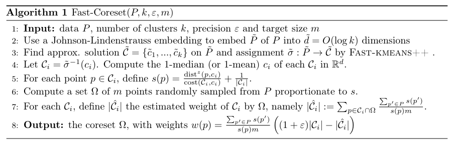
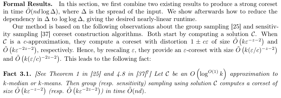
To turn Fact 3.1 into an algorithm, we use the quadtree-based Fast-kmeans++ approximation algorithm from [23], which has two key properties:
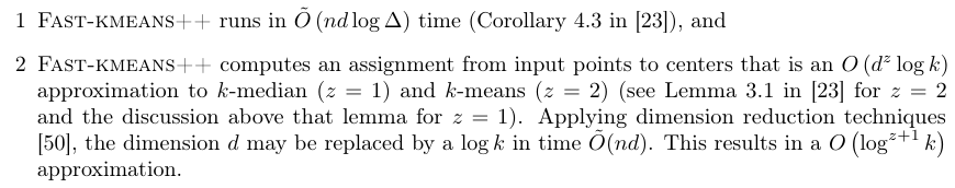
The second property is crucial for us: the algorithm does not only compute centers, but also assignments in O˜(nd log ∆) time. Thus, it satisfies the requirements of Fact 3.1 as a sufficiently good initial solution. We describe how to combine Fast-kmeans++ with sensitivity sampling in Algorithm 1 and prove in Section 8.1 that this computes an ε-coreset in time O˜(nd log∆):
Corollary 3.2. Algorithm 1 runs in time Oe (nd log ∆) and computes an ε-coreset for k-means
Furthermore, we generalize Algorithm 1 to other fast k-median approaches in Section 8.4.
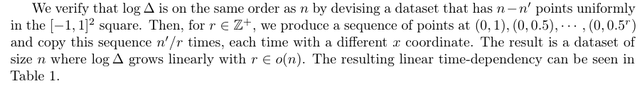
Thus, one can combine existing results to obtain an ε-coreset without an Oe(nk) time-dependency. However, this has only replaced the Oe(nd + nk) runtime by Oe(nd log ∆). Indeed, the spirit of the issue remains – this is not near-linear in the input size.
This paper is available on arxiv under CC BY 4.0 DEED license.
