Why Some Data Sampling Methods Fail (And Others Don’t)

Table of Links

Abstract and 1 Introduction

2 Preliminaries and Related Work

2.1 On Sampling Strategies

2.2 Other Coreset Strategies

2.3 Coresets for Database Applications

2.4 Quadtree Embeddings

3 Fast-Coresets

4 Reducing the Impact of the Spread

4.1 Computing a crude upper-bound

4.2 From Approximate Solution to Reduced Spread

5 Fast Compression in Practice

5.1 Goal and Scope of the Empirical Analysis

5.2 Experimental Setup

5.3 Evaluating Sampling Strategies

5.4 Streaming Setting and 5.5 Takeaways

6 Conclusion

7 Acknowledgements

8 Proofs, Pseudo-Code, and Extensions and 8.1 Proof of Corollary 3.2

8.2 Reduction of k-means to k-median

8.3 Estimation of the Optimal Cost in a Tree

8.4 Extensions to Algorithm 1

References

5.3 Evaluating Sampling Strategies

Theoretically guaranteed methods. We first round out the comparison between the Fast-Coreset algorithm and standard sensitivity sampling. Specifically, the last columns of Tables 4 and 5 show that the Fast-Coreset method produces compressions of consistently low distortion and that this

holds across datasets, m-scalar values and in the streaming setting. Despite this, Figure 1 shows that varying k from 50 to 400 causes a linear slowdown in sensitivity sampling but only a logarithmic one for the Fast-Coreset method. This analysis confirms the theory in Section 4 – Fast-Coresets obtain equivalent compression to sensitivity sampling but do not have a linear runtime dependence on k. We therefore do not add traditional sensitivity sampling to the remaining experiments.

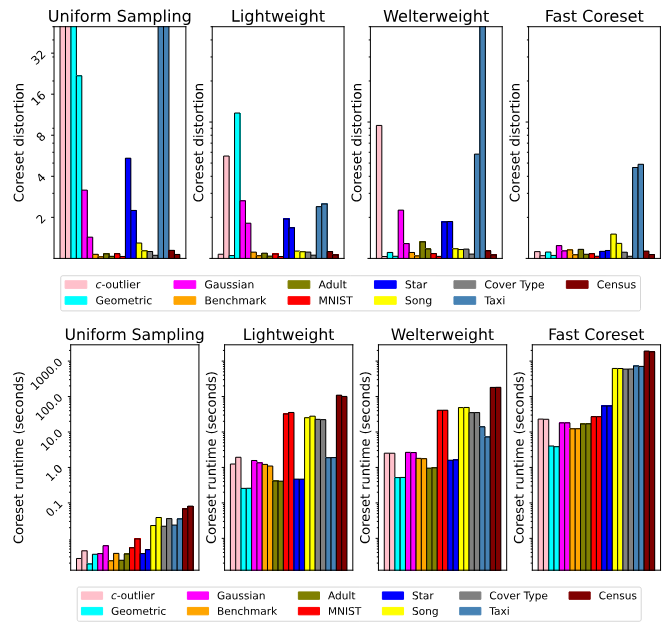
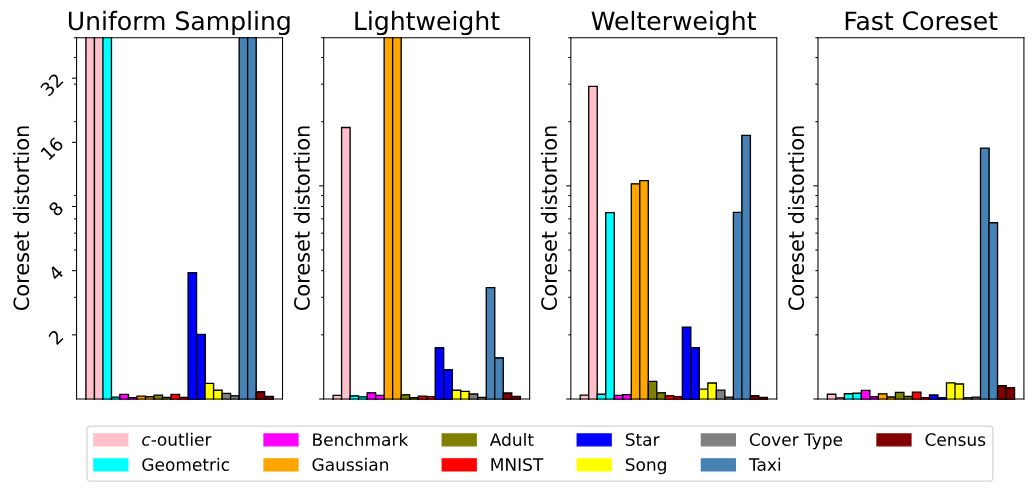
Speed vs. Accuracy. We now refer the reader to the remaining columns of Table 4 and to Figure 2, where we show the effect of coreset size across datasets by sweeping over m-scalar values. Despite the suboptimal theoretical guarantees of the accelerated sampling methods, we see that they obtain competitive distortions on most of the real-world datasets while running faster than Fast-Coresets in practice. However, uniform sampling breaks on the Taxi and Star datasets – Taxi corresponds to the 2D start locations of taxi rides in Porto and has many clusters of varied size while Star is the pixel values of an image of a shooting star (most pixels are black except for a small cluster of white pixels). Thus, it seems that uniform sampling requires well-behaved datasets, with few outliers and consistent class sizes.

To verify this, consider the results of these sampling strategies on the artificial datasets in Table 4 and Figure 2: as disparity in cluster sizes and distributions grows, the accelerated sampling methods

have difficulty capturing all of the outlying points in the dataset. Thus, Figure 2 shows a clear interplay between runtime and sample quality: the faster the method, the more brittle its compression.

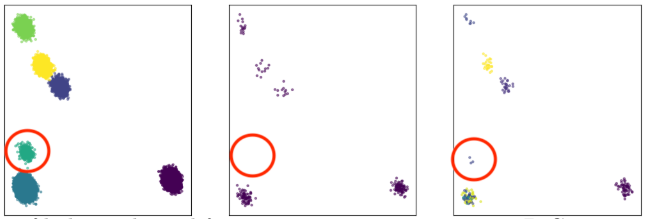
While uniform sampling is expected to be brittle, it may be less obvious what causes light- and welterweight coresets to break. The explanation is simple for lightweight coresets: they sample according to the 1-means solution and are therefore biased towards points that are far from the mean. Thus, as a simple counterexample, lightweight coresets are likely to miss a small cluster that is close to the center-of-mass of the dataset. This can be seen in Figure 3, where we show an example where the lightweight coreset construction fails on the Gaussian mixture dataset. Since the small, circled cluster is close to the center-of-mass of the dataset, it is missed when sampling according to distance from the mean.

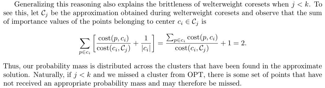
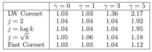
We evaluate the full extent of this relationship in Table 7, where we show the interplay between the welterweight coreset’s j parameter (number of centers in the approximate solution) and the Gaussian mixture dataset’s γ parameter (higher γ leads to higher class imbalance). We can consider this as answering the question “How good must our approximate solution be before sensitivity sampling can handle class imbalance?” To this end, all the methods have low distortion for small values of γ but, as γ grows, only Fast-Coresets (and, to a lesser extent, welterweight coresets for larger values of j) are guaranteed to have low distortion.

For completeness, we verify that these results also hold for the k-median task in Figure 4. There, we see that k-median distortions across datasets are consistent with k-means distortions. We show one of five runs to emphasize the random nature of compression quality when using various sampling schemas.

To round out the dataset analysis, we note that BICO performs consistently poorly on the coreset distortion metric[9], as can be seen in Table 6. We also analyze the Streamkm++ method across the artificial datasets in Table 9 with m = 40k and see that it obtains poor distortions compared to sensitivity sampling. This is due to Streamkm++’s required coreset size – logarithmic in n and exponential in d – being much larger than those for sensitivity sampling (sensitivity sampling coresets depend on neither parameter). We did not include Streamkm++ in tables 4, 5 due to its suboptimal coreset size, distortion and runtime.

Lastly, we point out that every sampling method performs well on the benchmark dataset, which is designed to explicitly punish sensitivity sampling’s reliance on the initial solution. Thus, we verify that there is no setting that breaks sensitivity sampling.

We lastly show how well these compression schemas facilitate fast clustering on large datasets in Table 8. Consider that a large coreset-distortion means that the centers obtained on the coreset poorly represent the full dataset. However, among sampling methods with small distortion, it may be the case that one consistently leads to the ‘best’ solutions. To test this, we compare the solution quality across all fast methods on the real-world datasets, where coreset distortions are consistent. Indeed, Table 8 shows that no sampling method leads to solutions with consistently minimal costs.

[9] We do not include BICO or Streamkm++ in Figures 2, 4, 5, as they do not fall into the O˜(nd) complexity class and are only designed for k-means.